In our previous post, Demystifying Pivot Tables in Excel with Examples – Part 1 , we had a brief discussion about what is Pivot Table, the salient features, stratification using Pivot Table and some use cases.
Following the previous post, we are here with some unknown yet useful features of Pivot that can enhance our work quality on a day-to-day basis. In this post we will be looking into the Pivot Charts, Filters and Slicers, Timelines and the feature of Calculated Fields in Pivot.
Pivot Charts:
 Pivot charts are the visual 2-Dimensional representation of the data. Pivot Table and Pivot charts are connected to each other.
Pivot Chart can be found under the analyse ribbon of PivotTable.
Tricks: Shortcut Keys for Pivot Chart- Alt + J + T + C or Alt + N + S + Z + C
Inserting a Pivot Chart:
1. Click any cell on the Pivot Table
2. Select the Pivot chart option from the analyze tab, in the Tools group.

3. Select OK and the pivot chart Appears.

Filters and Slicers in Pivot Chart:
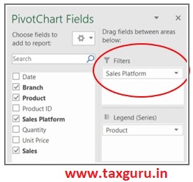
Filters are also available in pivot chart as available in Pivot Tables. It helps in the providing a pictorial representation of the required data as per the user’s needs.
- The filters can be applied by directly placing the data columns into the ‘Filter Field’ of the Pivot Chart Fields.
- Slicers can be applied for Pivot charts also. They can be found under the Filter Tab under Analyze Ribbon. The features of the slicers are similar to that found under the Pivot Table Features.

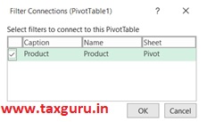
- In order to provide more convenience to the users, Excel has an option of connecting the slicers in common for both the Pivot Chart and Pivot Table sharing the same data. This is found in filter connection feature.
Calculated fields:
Often, once you create a Pivot table, there is a need you to expand your analysis and include more data/calculations as a part of it. If you need a new data point that can be obtained by using existing data points in the Pivot Table, you don’t need to go back and add it in the source data. Instead, you can use a Pivot Table Calculated Field to do this.

How to Add a Calculated Field?
1. From the Fields, Items & Sets option select the ‘Calculated Field’

2. A Dialogue Box ‘Insert Calculated Field’ would appear as below. Say suppose we need the tax collected on the sales.
a. Enter the name of the new field to be added in the Name Box, say GST.
b. In the Formula Box enter the calculation to be done. Here we assume the tax rate to be 18 %, so we insert the Sales field to the formula by selecting sales and clicking on the ‘Insert Field’.
c. Add the calculation “ *0.18 ” to the formula bar in order to get the GST value.
d. Select Add to insert the new field.

3. The New Calculated field would appear in the Pivot Table Fields and in the Pivot Table.

Things to Remember while using Calculated Field feature:
- You CAN NOT use references or named ranges while creating a Pivot Table Calculated Field. That would rule out a lot of formulas such as VLOOKUP, INDEX, and so on. However, you can use formulas that can work without references (such SUM, IF, COUNT, and so on..).
- You can use a constant in the formula. For example, if you want to know the forecasted sales where it is forecasted to grow by 10%, you can use the formula =Sales*1.1 (where 1.1 is constant).
- The order of precedence is followed in the formula that makes the calculated field. As a best practice, use parenthesis to make sure you don’t have to remember the order of precedence.
Inserting Timelines:
Pivot Table has the unique feature of identifying dates in the data and present them as Groups such as dates, Months, Quarters and Years. To make it even more advanced Excel provides the feature of Inserting timelines for a data where any such row is formatted as Date.

Inserting Timelines
Features of Timeline

1. Clear Filters: You can use this button to clear all filter.
2. Time Level: From time level option you can use four different time levels. You have days, months, quarters and years to use as time level.
3. Timeline: Use the timeline to filter dates for the period you want. You can filter dates for days, months, quarters and years. You also select more than a day, month, quarter & year but only in sequence.
Say we have a raw data consisting of sales for a period of 2 years for a restaurant operating across different cities. With the help of Timeline feature, the data can be filtered out for the necessary period as required by the end user.
The following will be the default pivot table for sales summary look like without applying the Timeline feature.

Applying the Timeline feature the sales summary can be filtered out for the required time period based on days, months, quarters and year. Following are some examples

Sources:
https://www.excel-easy.com/examples/pivot-chart.html
https://support.microsoft.com/en-us/office/create-a-pivotchart-c1b1e057-6990-4c38-b52b-8255538e7b1c
*****
Compiled by CA Narasimhan Elangovan with inputs from Nakul Pranav, team KEN & Co. Author can be reached at narasimhan@ken-co.in | https://www.ken-co.in.
Disclaimer : This publication contains information in summary form and is therefore intended for general guidance only. All information is provided in good faith. KEN & Co. makes no representation or warranty of any kind, express or implied, regarding the accuracy, adequacy, validity, reliability, availability, or completeness of any information provided. It is not intended to be a substitute for detailed research or the exercise of professional judgment.

Author Bio