In today’s scenario, proficiency in Excel is crucial. This comprehensive guide provides insights into Excel’s basic formulas, shortcut keys, important functions, and practical applications such as bank reconciliation and loan EMI calculation. You’ll also find tutorials on pivot tables, charts, and more.
Page Contents
Shortcut Keys in Excel
| Sr no | Function | Short Cut Key |
| 1 | Copy Formula | CTRL + C |
| 2 | Paste Formula | CTRL + V |
| 3 | Cut Formula | CTRL + X |
| 4 | Undo Formula | CTRL + Z |
| 5 | Copy Editing | CTRL + insert |
| 6 | Paste Editing | SHIFT + Insert |
| 7 | Save Selection | CTRL + s |
| 8 | Select entire region | CTRL + A |
| 9 | Print Navigation | CTRL + p |
| 10 | Bold a cell’s content | CTRL + B |
| 11 | Sum range | ALT + = |
| 12 | Insert hyperlink | CTRL + K |
| 13 | Select the whole column | CTRL + SPACE |
| 14 | Select the whole row | SHIFT + SPACE |
| 15 | Select table | SHIFT + CTRL + SPACE bar |
| 16 | Previous sheet | CTRL + Page Up |
| 17 | Next sheet | CTRL + Page Down |
| 18 | Go to last non-blank cell | CTRL + end |
| 19 | Go to previous sheet | CTRL + PgUp |
| 20 | Go to next sheet | CTRL + PgDn |
| 21 | Repeat whatever you did last | F4 |
| 22 | Calculate formulas | F9 |
| 23 | Hide row | CTRL + 9 |
| 24 | Hide column | CTRL + 0 |
| 25 | Unhide row | CTRL + SHIFT + 9 |
| 26 | Unhide column | CTRL + SHIFT + 0 |
| 27 | Sets/removes strikeout in current cell | CTRL + 5 |
| 28 | Single border around selected cells | CTRL + SHIFT + 7 |
| 29 | Sort | ALT + DS |
| 30 | Save as Excel | F12 |
| 31 | Opens print preview | CTRL + F2 |
| 32 | Activate next window | ALT + TAB |
| 33 | Close an excel workbook | crtl + F4 |
| 34 | Split screens | ALT + W + S |
| 35 | Show visual basic editor | ALT + F11 |
| 36 | Macro dialog | ALT + F8 |
| 37 | Apply/remove filter | ALT + DFF |
| 38 | Insert pivot table | ALT + NVT |
| 39 | Turn filter on or off | CTRL + SHIFT + L |
| 40 | Edit a cell, place cursor at the end | F2 |
| 41 | Fills down value from cell above | CTRL + D |
| 42 | Add a comment or Edit comment | SHIFT + F2 |
| 43 | Insert new sheet | SHIFT + F11 |
| 44 | Insert row | CTRL + + |
| 45 | Make chart/pivot chart | F11 |
| 46 | Edit a cell in Apple Macs | CTRL + U |
| 47 | Delete box(cell,row,column) | ALT + ED |
| 48 | Insert box(cell, row, column) | ALT + IE |
| 49 | Enter current date | CTRL + ; |
| 50 | Enter current time | CTRL + : |
General Basic Formulas
| Row Number | Sr No | Formula Name | Data — Column D | Data — Column E | Formulas | Answer |
| 4 | 1 | Multiplication | 10 | 15 | =D4*E4 | 150 |
| 5 | 2 | Addition | 10 | 15 | =D5+E5 | 25 |
| 6 | 3 | Subtraction | 10 | 15 | =D6-E6 | -5 |
| 7 | 4 | Division | 10 | 15 | =D7/E7 | 0.666666667 |
| 8 | 5 | Percentage | 10 | 15 | =D8/E8*100 | 67% |
| 9 | 6 | Average | 10 | 15 | =AVERAGE (D9,E9) | 12.5 |
| 10 | 7 | Count | 10 | 15 | =COUNT (D10,E10) | 2 |
| 11 | 8 | Sum Forumula | 10 | 15 | =SUM (D11:E11) | 25 |
| 12 | 9 | Days Calculator | 01-08-2022 | 27-08-2022 | =E12-D12 | 26 |
| 13 | 10 | Count Blank | 15 | =COUNTBLANK (D13:E13) | 1 | |
| 14 | 11 | Count Filled | 10 | 20 | =COUNTA (D14:E14) | 2 |
| 15 | 12 | Concatenate | Rohit | Raj | =CONCATENATE (D15,E15) | RohitRaj |
| 16 | 13 | Exact | Raj | Rohit | =EXACT (D16,E16) | FALSE |
| 17 | Rohit | Rohit | =EXACT (D17,E17) | TRUE | ||
| 18 | 14 | Match | Rohit | Veer | =MATCH (D18,D18:E18) | 1 |
| 19 | Veer | Veer | =MATCH (D19,D19:E19) | 2 | ||
| 20 | 15 | Proper | VEER | =PROPER(D20) | Veer | |
| 21 | veer | =PROPER (D21) | Veer | |||
| 22 | 16 | Upper | veer | =UPPER (D22) | VEER | |
| 23 | 17 | Lower | VEER | =LOWER (D23) | veer | |
| 24 | 18 | Right | Rajveer | 4 | =RIGHT (D24,E24) | veer |
| 25 | 19 | Left | Rajveer | 3 | =LEFT (D25,E25) | Raj |
| 26 | 20 | Middle | Rajveer | 3 | =MID (D26,1,E26) | Raj |
| 27 | 21 | Small | 10 | 15 | =SMALL (D27:E27,1) | 10 |
| 28 | 22 | Large | 10 | 15 | =LARGE (D28:E28,1) | 15 |
| 29 | 23 | Minimum | 10 | 15 | =MIN (D29,E29) | 10 |
| 30 | 24 | Maximum | 10 | 15 | =MAX (D30,E30) | 15 |
| 31 | 25 | Product | 10 | 15 | =PRODUCT (D31,E31) | 150 |
| 32 | 26 | Sum Product | 10 | 15 | =SUMPRODUCT (D32:E32,D33:E33) | 325 |
| 33 | 10 | 15 | ||||
| 34 | 27 | Trim | Raj Rohit | =TRIM (D34) | Raj Rohit | |
| 35 | 28 | Find | Rajveer | e | =FIND (E35,D35,1) | 5 |
| 36 | 29 | Replace | Veer | a | =REPLACE (D36,7,2,E36) | Veera |
| 37 | 30 | Search | Rajveer | v | =SEARCH (E37,D37,1) | 4 |
Important Formulas
Row Number |
Sr No |
Formula Name |
Data — Column D |
Data — Column E |
Formula |
Answer |
41 |
1 |
Hide the Sensitive Data |
Rajveer |
veer (hidden require) |
=LEFT (D41,3) &”****” |
Raj**** |
42 |
Hide the Sensitive Data |
Rajveer |
Raj (hidden require) |
=”***”& RIGHT (D42,4) |
***veer |
|
43 |
2 |
Sum Running Total Formula |
100 |
150 |
=SUM($D$43:E43) |
250 |
44 |
100 |
150 |
=SUM($D$43:E44) |
500 |
||
45 |
100 |
150 |
=SUM($D$43:E45) |
750 |
||
46 |
100 |
150 |
=SUM($D$43:E46) |
1000 |
||
47 |
3 |
Sum If Formula |
Rohit |
100 |
=SUMIF ($D$47:$ D$51,”Rohit”, $E$47:$E$51) |
525 |
48 |
Rohit |
175 |
||||
49 |
Veer |
150 |
=SUMIF (D47:D51,”Veer”,E47:E51) |
270 |
||
50 |
Veer |
120 |
||||
51 |
Rohit |
250 |
||||
52 |
4 |
Round the Value to Zero Decimal Place |
23.458 |
=ROUND (E52,0) |
23 |
|
53 |
5 |
Round the Value to One Decimal Place |
23.458 |
=ROUND (E53,1) |
23.5 |
|
54 |
6 |
Round the Value to Multiple of 10 |
23.458 |
=ROUND (E54,-1) |
20 |
|
55 |
7 |
Round the Value to the Next Integer Number |
23.458 |
=ROUNDUP (E55,0) |
24 |
|
56 |
8 |
Round up the Value to 1 Decimal Place |
23.458 |
=ROUNDUP (E56,1) |
23.5 |
|
57 |
9 |
Round up the Value to Next Multiple of 10 |
23.458 |
=ROUNDUP(E57,-1) |
30 |
|
58 |
10 |
Round the value to the Previous Integer Number |
23.458 |
=ROUNDDOWN (E58,0) |
23 |
|
59 |
11 |
Round down the Value to 1 Decimal Place |
23.458 |
=ROUNDDOWN (E59,1) |
23.4 |
|
60 |
12 |
Round down the Value to Previous Multiple of 10 |
23.458 |
=ROUNDDOWN (E60,-1) |
20 |
|
61 |
13 |
Information about your Computer |
Current directory |
=INFO (“directory”) |
C:\Users\Dinesh \Documents\ |
|
62 |
14 |
Information about your Computer |
Number of active worksheets |
=INFO (“numfile”) |
44 |
|
63 |
15 |
Information about your Computer |
Cell currently in the top left of the window |
=INFO (“origin”) |
$A:$A$140 |
|
64 |
16 |
Information about your Computer |
Operating system |
=INFO (“osversion”) |
Windows (32-bit) NT 6.02 |
|
65 |
17 |
Information about your Computer |
Recalculation mode |
=INFO (“recalc”) |
Automatic |
|
66 |
18 |
Information about your Computer |
Excel version |
=INFO (“release”) |
14.0 |
|
67 |
19 |
Information about your Computer |
Name of system. (PC or Mac) |
=INFO (“system”) |
pcdos |
|
68 |
20 |
EMI Formula |
Loan |
100000 |
=PMT (E69/12,E70,E68) |
8745.15 |
69 |
Rate Per Annum |
9% |
||||
70 |
Tenure in Months |
12 |
||||
71 |
21 |
V Look up Formula |
Raj |
1500 |
Search Amount of Veer |
3500 |
72 |
Rohit |
2000 |
Veer |
|||
73 |
Rohit |
2500 |
=VLOOKUP (F72,D71:E75,2,0) |
|||
74 |
Raj |
3000 |
||||
75 |
Veer |
3500 |
||||
76 |
22 |
H Look up Formula |
Raj |
Veer |
Veer |
2000 |
77 |
1500 |
2000 |
=HLOOKUP (F76,D76:E77,2,0) |
|||
78 |
23 |
2 Ways Lookup using V Lookup |
Name |
Jan |
Feb |
200 |
79 |
Raj |
1000 |
200 |
|||
80 |
Rohit |
1200 |
400 |
|||
81 |
Search Shyam Amount in Feb Month |
=VLOOKUP (D82,D78:F80,MATCH (E82,D78:F78,0)) |
||||
82 |
Raj |
Feb |
||||
83 |
24 |
Ceiling Formula |
1000.52 |
0.05 |
=CEILING (D83,E83) |
1000.55 |
84 |
1000.58 |
0.05 |
=CEILING (D84,E84) |
1000.6 |
||
85 |
25 |
Remove Unwanted Words/ Characters |
1234-5678-1234 |
– |
=SUBSTITUTE (D85,E85,””) |
123456781234 |
86 |
5678*1234*5678 |
* |
=SUBSTITUTE (D86,E86,””) |
567812345678 |
||
87 |
1234/5678/1234 |
/ |
=SUBSTITUTE (D87,E87,””) |
123456781234 |
||
88 |
1234+5678+1234 |
+ |
=SUBSTITUTE (D88,E88,””) |
123456781234 |
||
89 |
26 |
Join First Name & Last Name |
Raj |
Rohit |
=D89&” “&E89 |
Raj Rohit |
90 |
Rohit |
Raj |
=D90&” “&E90 |
Rohit Raj |
||
91 |
Rohit |
Veer |
=D91&” “&E91 |
Rohit Veer |
||
92 |
Veer |
Rohit |
=D92&” “&E92 |
Veer Rohit |
||
93 |
27 |
Split First Name & Surname |
Rohit Veer |
=LEFT (D93, SEARCH (“”,D93)*5) |
Rohit |
|
94 |
Veer Rohit |
=RIGHT (D94,LEN(D94)-SEARCH (“”,D94,5)) |
Rohit |
|||
95 |
Rohit Veer |
=RIGHT (D95,LEN(D95)-SEARCH (“”,D95,6)) |
Veer |
|||
96 |
Veer Rohit |
=LEFT (D96, SEARCH (“”,D96)*5) |
Veer |
|||
97 |
28 |
Convert Numbers to Roman |
7 |
=ROMAN(D97,1) |
VII |
|
98 |
9 |
=ROMAN(D98,1) |
IX |
|||
99 |
12 |
=ROMAN(D99,1) |
XII |
|||
100 |
20 |
=ROMAN(D100,1) |
XX |
|||
101 |
29 |
Get the Desired Number of Character |
Raj Rohit |
3 |
=LEFT(D101,E101) |
Raj |
102 |
Rohit Raj |
5 |
=LEFT(D102,E102) |
Rohit |
||
103 |
30 |
Get the Desired Number of Character |
Rohitveer |
4 |
=RIGHT(D103,E103) |
veer |
104 |
VeerRohit |
5 |
=RIGHT(D104,E104) |
Rohit |
||
105 |
31 |
Count if Formula |
Names |
Days Present/Absent |
||
106 |
Veer Day-1 |
P |
Veer Counting Days |
Present/Absent Days of Ram |
||
107 |
Veer Day-2 |
P |
=COUNTIF (E106:E108,”P”) |
2 |
||
108 |
Veer Day-3 |
A |
=COUNTIF (E106:E108,”A”) |
1 |
||
109 |
Rohit Day-1 |
P |
Rohit Counting Days |
Present/Absent Days of Shyam |
||
110 |
Rohit Day-2 |
P |
=COUNTIF (E109:E111,”P”) |
3 |
||
111 |
Rohit Day-3 |
P |
=COUNTIF (E109:E111,”A”) |
0 |
||
112 |
32 |
Count Length of Number of Words |
Raj |
=LEN(D112) |
3 |
|
113 |
Rohit |
=LEN(D113) |
5 |
|||
114 |
Veer |
=LEN(D114) |
4 |
|||
115 |
Rohitveer |
=LEN(D115) |
9 |
|||
116 |
33 |
Count Cell that start with Specific Alphabet |
A-Raj |
B-Rohit |
Count Alphabet Starts with A |
3 |
117 |
B-Rohit |
A-Raj |
A |
|||
118 |
A-Veer |
C-Veer |
=COUNTIF (D116:E118,”*A*”) |
|||
119 |
34 |
Count Cell that ends with Specific Alphabet |
Raj-A |
Rohit-B |
Count Alphabet Starts with B |
2 |
120 |
Raj-A |
Rohit-A |
B |
|||
121 |
Veer-A |
Veer-B |
=COUNTIF (D119:E121,”*B”) |
|||
122 |
35 |
Current Date & Time Formula |
=NOW() |
31-03-2024 20:44 |
||
123 |
36 |
Separate Date & Time |
24-08-2022 12:10 |
=INT(D123) |
24-08-2022 |
|
124 |
=D123-G123 |
12:10:00 |
||||
125 |
26-08-2022 21:20 |
=INT(D125) |
26-08-2022 |
|||
126 |
=D125-G125 |
21:20:00 |
||||
127 |
37 |
Separate Day, Month & Year from Date |
24-08-2022 |
=DAY(D127) |
24 |
|
128 |
=MONTH(D127) |
8 |
||||
129 |
=YEAR(D127) |
2022 |
||||
130 |
38 |
Time Calculation |
Old Time |
Addition in Hours |
New Time |
|
131 |
01:20 |
05:00 |
=D131+E131 |
06:20 |
||
132 |
04:40 |
03:00 |
=D132+E132 |
07:40 |
||
133 |
08:30 |
04:00 |
=D133+E133 |
12:30 |
||
134 |
15:20 |
05:00 |
=D134+E134 |
20:20 |
||
135 |
39 |
Get Day Name by |
12-08-2022 |
=TEXT (D135,”DDDD”) |
Friday |
|
136 |
15-08-2022 |
=TEXT (D136,”DDDD”) |
Monday |
|||
137 |
39 |
Date |
18-08-2022 |
=TEXT(D137,”DDDD”) |
Thursday |
|
138 |
24-08-2022 |
=TEXT(D138,”DDDD”) |
Wednesday |
|||
139 |
40 |
Get Date in Desired Formats |
12-08-2022 |
“DD MMM YYYY” |
=TEXT (D139,”DD MMM YYYY”) |
12 Aug 2022 |
140 |
15-08-2022 |
“DD-MM-YYYY” |
=TEXT(D140,”DD-MM-YYYY”) |
15-08-2022 |
||
141 |
18-08-2022 |
“DD MMM YY” |
=TEXT(D141,”DD MMM YY”) |
18 Aug 22 |
||
142 |
41 |
Calculate Month in Numbers & in Words from Date |
Date |
Month in Numbers |
||
143 |
12-04-2022 |
=MONTH(D143) |
4 |
|||
144 |
Month in Words |
|||||
145 |
18-07-2022 |
=TEXT (D145,”MMMM”) |
July |
|||
146 |
42 |
Age Calculator |
Age |
Birth Date |
=(TODAY()-E148)/365.25 |
32.50 |
147 |
Years Lived |
=DATEDIF (E148,TODAY(),”Y”) |
32.00 |
|||
148 |
Months Lived |
29-09-1991 |
=DATEDIF (E148,TODAY(),”YM”) |
6.00 |
||
149 |
Days Lived |
=DATEDIF (E148,TODAY(),”MD”) |
2.00 |
|||
150 |
43 |
Rank Position High to Low |
25 |
=RANK (D150,$D$150:$D$152) |
2 |
|
151 |
18 |
=RANK (D151,$D $150:$D$152) |
3 |
|||
152 |
40 |
=RANK (D152,$D $150:$D$152) |
1 |
|||
153 |
44 |
Rank Position Low to High |
25 |
=RANK (D153,$D$153:$D$155,1) |
2 |
|
154 |
42 |
=RANK (D154,$D$153:$D$155,1) |
3 |
|||
155 |
18 |
=RANK (D155,$D$153: $D$155,1) |
1 |
|||
156 |
45 |
Repeated Formulas |
Data-1 |
Number of Repeats |
Repeated Data |
|
157 |
Raj |
3 |
=REPT (D157,E157) |
RajRajRaj |
||
158 |
Veer |
2 |
=REPT (D158,E158) |
VeerVeer |
||
159 |
* |
5 |
=REPT (D159,E159) |
***** |
||
160 |
15 |
4 |
=REPT (D160,E160) |
15151515 |
||
EMI Calculation Formula & Loan Calculator
| EMI Calculation Formula & Loan Calculator | |||
| Loan | 100000 | ||
| Rate | 9% | Per Annum | |
| Tenure | 12 | Months | |
| EMI Formula | 8745.15 | Answer | Formula=PMT (B3/12,B4,B2) |
–
| Months | Opening Bal. | Interest | EMI | Closing Bal. |
| 1 | 1,00,000.00 | 750.00 | 8,745.15 | 92,004.85 |
| 2 | 92,004.85 | 690.04 | 8,745.15 | 83,949.74 |
| 3 | 83,949.74 | 629.62 | 8,745.15 | 75,834.22 |
| 4 | 75,834.22 | 568.76 | 8,745.15 | 67,657.83 |
| 5 | 67,657.83 | 507.43 | 8,745.15 | 59,420.11 |
| 6 | 59,420.11 | 445.65 | 8,745.15 | 51,120.61 |
| 7 | 51,120.61 | 383.40 | 8,745.15 | 42,758.87 |
| 8 | 42,758.87 | 320.69 | 8,745.15 | 34,334.42 |
| 9 | 34,334.42 | 257.51 | 8,745.15 | 25,846.78 |
| 10 | 25,846.78 | 193.85 | 8,745.15 | 17,295.48 |
| 11 | 17,295.48 | 129.72 | 8,745.15 | 8,680.05 |
| 12 | 8,680.05 | 65.10 | 8,745.15 | – |
| Formulas | =+E18 | =+B19*$B$3/$B$4 | =-$B$5 | =+B19+C19-D19 |
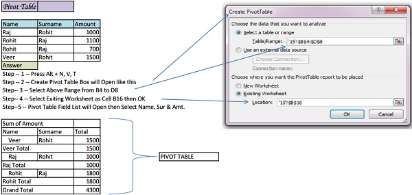
Pivot Table
–

–

Bank Reconciliation in Excel
| Bank Book of XXXX Bank for the Month of January, 2020 | |||||
| Date | Particulars | Cheque No Deposit | Withdrawal | Closing Balance | |
| Opening Balance as per our Records | 512100 | ||||
| 31-12-2019 | Cheuqe Deposit | xxxxxx | 6500 | 518600 | |
| 31-12-2019 | Cheuqe Deposit | xxxxxx | 302400 | 821000 | |
| 31-12-2019 | Cheuqe Withdrawl | xxxxxx | 0 | 815000 | 6000 |
| 02-01-2020 | Cheuqe Deposit | xxxxxx | 1020600 | 1026600 | |
| 07-01-2020 | Cheuqe Deposit | xxxxxx | 104700 | 921900 | |
| 07-01-2020 | Cheuqe Deposit | xxxxxx | 55200 | 977100 | |
| 08-01-2020 | Cash Withdrawl | xxxxxx | 25200 | 951900 | |
| 09-01-2020 | Cash Deposit | xxxxxx | 95100 | 1047000 | |
| 09-01-2020 | Cash Deposit | xxxxxx | 7735 | 1054735 | |
| 15-01-2020 | Cheuqe Deposit | xxxxxx | 302400 | 1357135 | |
| 15-01-2020 | Cheuqe Withdrawl | xxxxxx | 0 | 800000 | 557135 |
| 20-01-2020 | Cheuqe Deposit | xxxxxx | 1020500 | 1577635 | |
| 20-01-2020 | Cheuqe Withdrawl | xxxxxx | 102000 | 1475635 | |
| 25-01-2020 | Cheuqe Deposit | xxxxxx | 51000 | 1526635 | |
| 29-01-2020 | Cheuqe Withdrawl | xxxxxx | 24000 | 1502635 | |
| 29-01-2020 | Cheuqe Deposit | xxxxxx | 95000 | 1597635 | |
| 31-01-2020 | Cheuqe Deposit | xxxxxx | 75000 | 1522635 | |
| 01-02-2020 | Cheuqe Deposit | xxxxxx | 13000 | 1535635 | |
| Closing Balance as per our Records | 1535635 | ||||
2 Steps for Bank Reconciliation in Excel
1) Prepare your Bank Book in Excel Format, As Prepared here.
2) Insert Bank Clearing Date by referring from Bank Statement in H Column & insert Formulas in I & J Column
3) Prepare Bank Reconciliation Summary
| Bank Reconciliation Summary | |
| Closing Bal. as per our Record | 1535635 |
| Less :- Uncleared Deposits | 114500 |
| Add :- Uncleared Withdrawls | 99000 |
| Closing Bal. as per Statement | 1520135 |
–
| Bank Clearing Date | Uncleared Deposits | Uncleared Withdrawal |
| 6500 | 0 | |
| 03-01-2020 | =IF(H8>0,””,D8) | =IF(H8>0,””,E8) |
| 03-01-2020 | =IF(H9>0,””,D9) | =IF(H9>0,””,E9) |
| 05-01-2020 | ||
| 10-01-2020 | ||
| 10-01-2020 | ||
| 08-01-2020 | ||
| 09-01-2020 | ||
| 09-01-2020 | ||
| 18-01-2020 | ||
| 18-01-2020 | ||
| 23-01-2020 | ||
| 23-01-2020 | ||
| 28-01-2020 | ||
| 0 | 24000 | |
| 95000 | 0 | |
| 0 | 75000 | |
| 13000 | 0 | |
| Total | 114500 | 99000 |
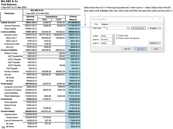
How to Remove “Cr” & “Dr” from exported Tally in Excel Format
Kindly Refer to
Privacy Policy &
Complete Terms of Use and Disclaimer.


Dear sir,
I would like to join Excel Course. I am interested to get Excel knowledge from you.