Summary: Depreciation spreads the cost of a tangible asset over its useful life, helping match the expense with the revenue it generates. In the Written Down Value (WDV) method, commonly used for assets like machinery, depreciation is higher in the early years. However, when calculating depreciation for assets purchased mid-year, a proportionate approach must be followed to prevent discrepancies in scrap value. The simple division method, while commonly used, may lead to errors by not accounting for unapportioned depreciation. A more accurate method involves calculating depreciation for the remaining life of the asset, adjusting for unapportioned depreciation from previous years. While this method provides more precision, especially for matching desired scrap values, it is complex to apply. Therefore, understanding the formula derivation, such as the depreciation rate and its relation to compounding factors, is crucial. Proper application of these concepts ensures accurate depreciation and avoids unintended deviations in asset values over time.
The most appropriate way of calculating and apportioning the depreciation of an asset over its useful life, in case of “Written Down Value Method”.
DEPRECIATION
Depreciation allocates the cost of tangible asset over its useful life. In accounting, the matching principle states that expenses should be recorded in the same period as the revenues they help generate. Depreciation allows companies to match the expense of using an asset with the revenue that the asset generates over its useful life. Written Down Value (WDV) method (a.k.a. Diminishing Value method) is one of the most commonly used methods of depreciation, especially for those assets that lose value more quickly in their early years, like machinery and vehicles.
Let us begin with a quick example:
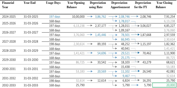
| Cost of the Asset | 10,00,000 | Since, the asset has not been used for full year in the year 1, we usually take a proportionate amount of depreciation in the year 1, based on number of usage days. In the current example, the asset has been used for 197 days in the year 1 and therefore, the total depreciation for the full year 3,86,762 has been split to 2,08,746 representing the depreciation amount for 197 days. |
| Useful Life | 8 Years | |
| Scrap(%) | 2% | |
| Scrap Value | 20,000 | |
| Date of Purchase | 15-09-2024 |
So, based on the above inputs, the depreciation rate can be calculated
| Financial Year | Usage Days | Year End | Year Opening Balance | Depreciation | Year Closing Balance |
| 2024-2025 | 197 days | 31-03-2025 | ₹10,00,000 | ₹2,08,746 | ₹7,91,254 |
| 2025-2026 | 365 days | 31-03-2026 | ₹7,91,254 | ₹3,06,027 | ₹4,85,227 |
| 2026-2027 | 365 days | 31-03-2027 | ₹4,85,227 | ₹1,87,668 | ₹2,97,559 |
| 2027-2028 | 366 days | 31-03-2028 | ₹2,97,559 | ₹1,15,085 | ₹1,82,475 |
| 2028-2029 | 365 days | 31-03-2029 | ₹1,82,475 | ₹70,574 | ₹1,11,900 |
| 2029-2030 | 365 days | 31-03-2030 | ₹1,11,900 | ₹43,279 | ₹68,621 |
| 2030-2031 | 365 days | 31-03-2031 | ₹68,621 | ₹26,540 | ₹42,081 |
| 2031-2032 | 366 days | 31-03-2032 | ₹42,081 | ₹16,275 | ₹25,806 |
| 2032-2033 | 168 days | 31-03-2033 | ₹25,806 | ₹4,594 | ₹21,212 |
⇓
The actualdesired scrap value is 20,000. But the scrap value that has been derived by depreciating the asset is 21,139. A clear deviation of
1,139 which is 6% of the actual scrap value is observed.
Did you notice, what just happened. At the end of the useful life of the asset, the scrap value is not as we desired at the beginning of the year. Try guessing what went wrong in the above calculation.
Let me explain, the rate we apply on the opening WDV is an annual rate. When ever we apply such rate on WDV of an asset, the result will be an amount that represents depreciation for one complete year. The apportionment of such amount derived has to be appropriate. So, it is crucial to understand, how the application of rate of depreciation works and how to apportion the depreciation in an appropriate manner, so that we do not commit the mistake that we did in the above example leading a wrong scrap value of the asset at the end of it’s useful life.
| When an asset is purchased in the middle of an year, it is appropriate to apportion the depreciation of year 1 based on the number of usage days in year 1. But the way of apportionment does also matter. The general way of apportionment is done as shown in the initial example. The rate will be applied on the opening WDV of the asset. We will obtain an amount that represents depreciation for a complete year. Later, the same will be apportioned using the simple division method. | Such way of apportionment is not appropriate, and will have effect on the depreciation amount that we calculate for future years. Because, the rate being applied results an amount which is depreciation for one complete year, as the rate we use will be usually an annual rate. For instance, in the example we have taken, the asset is purchased in the month of September. When we apply the rate on the opening WDV of the asset, the resulted amount represents depreciation till September of next year. |
It has to be noted that, if the total amount of depreciation has been apportioned using simple division, based on number of days used in year 1, then in the year 2, the rate directly can not be applied on the opening WDV as on year beginning. The unapportioned part of the depreciation amount that we have calculated in the year 1 is still not considered. After deducting the remaining part of year 1 depreciation from the opening WDV, we will get some balance as on September. The rate for calculating depreciation for the year 2 can be applied now, and then it gives us depreciation for one full year, again we have to apportion form September to March of the second financial year.
| In simple terms, the depreciation for the year 2 should be the sum of:
a) Unapportioned part of depreciation that we have calculated in the year 1. b) Proportionate amount of depreciation that we calculated in year 2 in September by applying the rate on the WDV after deducting the complete amount of depreciation till September that we have calculated in the year 1. |
In other words, the WDV on which we apply the rate in year 2 will be the same that we used in year 1, till September month. After
September, the WDV changes. This cycle has to be continued till the end of the useful life of the asset to get an accurate amount of desired scrap value of the asset. The above concept can be understood clearly with help of the below example:
By using the above method of apportionment, the desired scrap value at the end of the useful life of the asset has been achieved. If you observe carefully, you might have noticed one thing. The depreciation amount and the closing WDV at the end of each that we have calculated, using the simple division method, is exactly same as the depreciation amount and closing WDV, that we calculated using the second method (A very little deviation in case of leap year will be observed. However, the same will get automatically adjusted in the immediate next financial year). Difference can be observed only in the last financial year. Try guessing what could be the possible reason.
Let me explain,
Depreciation for the first will be same in both methods since there will be no concept of unapportioned part of previous year’s depreciation, in the second method that we used. Further, do you agree, if I say, that the formula that we use for calculating the depreciation from the year two, is nothing but the “simplified version” of the formula that we use in calculating the depreciation amount in the second method.
The formula for calculating depreciation for the year 2 as per the simple division method will be:
Where,
D2 is the depreciation for year 2.
Y1 is the WDV as at end of Year 1.
R is the Rate of Depreciation.
Let us see understand, how the complex formula that we used in method two, once simplified, is exactly same as the formula that we used in simple division method.
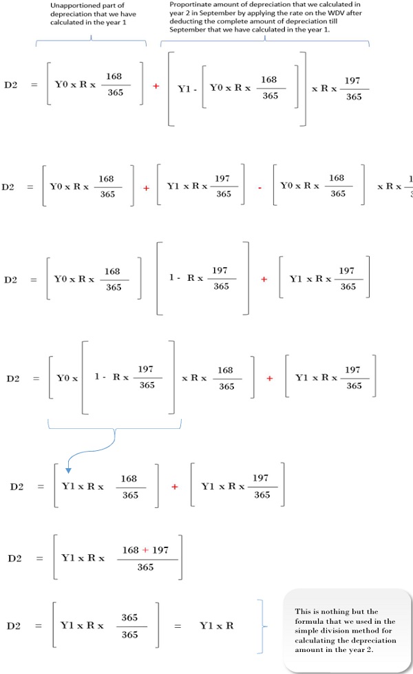
Where, Y0 is the WDV at the beginning of the year 1.
You may ask, if the formulas that we used in both the methods are same, then why did the scrap value at the end of the useful life of the asset is not matching?
In the last financial year, the formula that we used in the second method will be changing. This is because the depreciation will be the mere unapportioned part of the previous year’s depreciation and not the summation of two components that we have gone through till now.
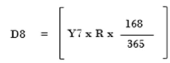
The formula for calculation of depreciation amount for the last financial as per the simple division method will be:
The formula for calculation of depreciation amount for the last financial as per the second method will be:
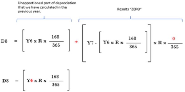
It is apparent that, in the simple division method the rate is being applied on “Y7” which is opening WDV for that last financial year which is year 8. In the second method the rate will be first applied on the “Y6” that is, opening WDV of year 7, for the purpose of finding the unapportioned part of depreciation that is calculated in the year 7.
The only one thing that the simple division method is missing is:
It does not care about the unapportioned part of depreciation of the financial that is immediately preceding to the last financial year. Instead it calculates the deprecation by applying the rate on the opening WDV in the last financial year which results a lesser depreciatin amount. And therefore, the value of the asset at its end of the useful life gets deviated from the actual desired scrap value.
I hope you are with me till now in this journey of exploration. Though the simple division method and the second method of apportionment gives us the same results, it does not happen in the last financial year. The second method is giving us the accurate amount of desired scrap value. However, even after finding and understanding all the above derivations and methods that gives us the desired scrap value, I still do not prefer or conclude the second method of apportionment as the most appropriate method of apportionment of depreciation.
Let me demonstrate why,
Reason 1: Though we have achieved the desired scrap value of the asset at the end of it’s useful life, it is clear that the calculation of depreciation becomes complicated while doing the apportionment.
Reason 2: This is the main and important one. The application of a formula should be satisfying the purpose of deriving the same. Therefore, the derivation of the formula for rate has to be first understood before applying the rate for calculating the depreciation.
Therefore, to know the most appropriate method of apportionment of depreciation of an asset, a clear understanding of the derivation and application of the rate of depreciation is required.
The formula for calculating the rate of depreciation is shown as below:
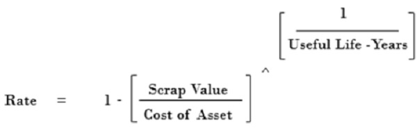
Understanding the derivation of the above formula is crucial. Let me explain you the way the above formula has come. To understand the concept, you should be aware of compounding.
Therefore, let us understand how compounding works first, and what is meant by the “Compounding Factor“.
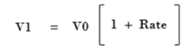
Where V1 indicates the Value at the end of the Year 1 and the V0 is nothing but the Value at the beginning of the period and the rate used is generally assumed as on per annum basis.
If you want to calculate the value at the end of the Year 2, you do it as shown below:
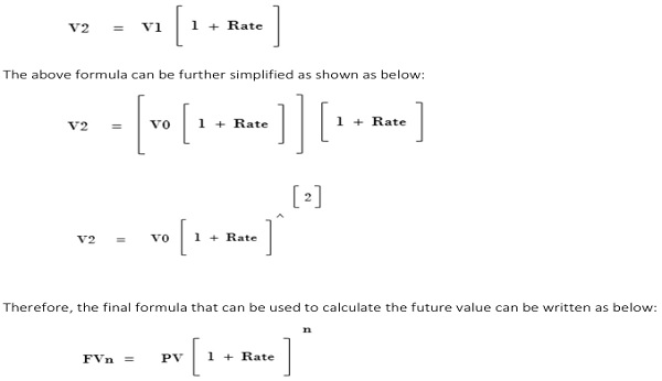
We can call the below as the compounding factor:
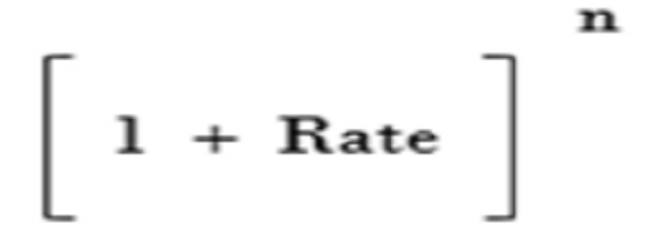
When the compounding factor is multiplied to the present value, the future value can be determined.
The very important thing to understand about the compounding factor:
The term “n” in the compounding factor indicates the periodic frequency of compounding. In simple terms, number of compounding periods.
The “Rate” we use to compound should be according to the “n” we take.
In the above derivation, we are compounding for years and therefore the rate we used is an annual rate.
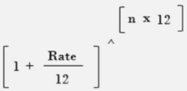
If we intend to compound at the end of each month, the number of compounding periods would be 12 times of the “n” we have taken above.
And then it does not stop there, the rate we used to compound shall also be changed to the monthly rate. It can be done simply by dividing the annual rate by 12.
What it does is simply, break down the annual rate to monthly rate and then compound 12 times with such broken down rate, in a year.-
Therefore, the rate we use to compound depends on periodic frequency of compounding.
You may think that why am I explaining all the above and how above things are related depreciation.
Well, let me take you to the next level of our journey in this exploration.
| The value we achieve in compounding is an amount that is accumulated with interest for each occurrence of compounding. But in the context of Depreciation and WDV method, at the end of the period, we need to achieve some amount that is the end compressed value of the asset, nothing but the scrap value of the asset at the end of it’s useful life. | In simple terms, as we go forward in time, the value keeps on accumulating in case of compounding, whereas it keeps on diminishing in case of depreciation. The concept of depreciating an asset under WDV method is exactly opposite to the concept of compounding. |
Now, we need something similar to the compounding factor, but it should diminish or compress the value rather than compounding the
value. This can be achieved just by replacing the “+” sign with “-” sign in the compounding factor.
Let me name it as the “Compressing Factor” and it looks like below:
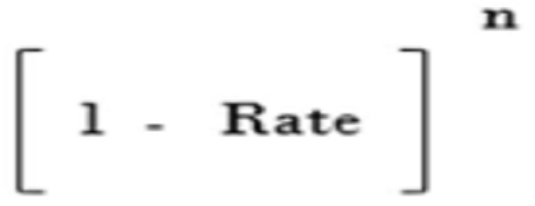
The compressed end value of the asset, nothing but the scrap value at the end of it’s useful life can be determined by multiplying the compressing factor to the cost of the asset at the beginning of the period.
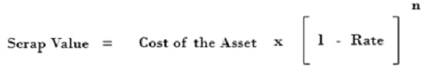
The difference between the compressed value of the asset at the end of each period and the value at the beginning of such period is nothing but the “Depreciation” for that particular period.
Let us understand this using the below example:
| Asset Cost | 10,00,000 |
| Depreciation Rate | 26% |
| Useful Life | 10 |
Now, using the compressing factor we can determine the end value of the asset that is nothing but the scrap value.
Scrap Value of the above asset at the end of 10th year will be: 1,00,000x(1-26%)”10
Resulting 50,000
In practical world, we do not know the depreciation rate of a particular asset, we have to determine the same based on various inputs like the cost of the asset, useful life of that asset and the scrap value of the same at the end of it’s useful life. So, we can use some mathematical operations to the above formula that we used to determine the scrap value of the asset, it looks like below:
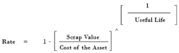
The rate we determined using above formula is already adjusted based on terms of the compressing period.
It means, if the useful life is taken in years, the rate obtained represents an annual rate.
If the useful life is taken in months, the rate obtained represents a monthly rate.
Applying the compression factor with the power “1”, to the opening written down value of the asset results the written down value at the end of the period. If the rate is used is an annual rate it resulted value represents the written down value at the year end. If the rate used is a monthly rate, the resulted value represents the written down value at the month end. Further, the extent to which this compression takes place can be controlled using the power of the compressing factor. If the power of the compressing factor that we used is 2 and the rate used is an annual rate, the resulted value represents the written down value of the asset at the end of second year. The same way, we can also if we use power as “0.5” the result would be the written down value of the asset at the end of six months. So, the extent till when the asset has to depreciated can be decided using the power of the compressing factor.
The method of using the compression factor for depreciating an asset can be understood using below example:
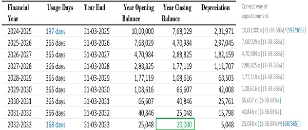
By using the compression factor and the number of days used in the year 1, we found the value at the end of the year 1, that is 7,68,029. The extent of the amount, to which the value of the asset has been compressed is nothing but the depreciation for the year 1. This value can be directly used for compressing the value of the asset further. Doing so, we have achieved our desired scrap value of 20,000 at the end of the useful life of the asset.
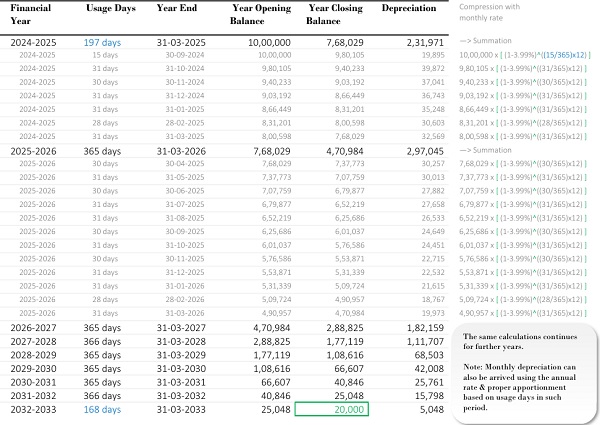
Most of the companies prefer calculating depreciation on a monthly basis. In such case, a monthly rate can be calculated as we have discussed earlier. The annual rate will be broken down to a monthly rate, and then compression takes place on a monthly basis. The above example can be modified as below:
Rate of Depreciation
1-(20,000/10,00,000)^(1/(8*12)) 3.99%per month
The compression method used above in calculating the rate of depreciation provides 100% satisfaction in terms of aligning with the derivation of the formula. This method ensures that the depreciation rate is applied accurately and consistently, offering a solid foundation for apportioning depreciation in a manner that fully complies with the mathematical and financial principles behind the Written Down Value method. With this approach, you can be confident that the depreciation calculations are precise and fully in line with the expected outcomes of the formula.
Thank you for sticking with me on this journey! I sincerely appreciate your patience and the effort you’ve invested in exploring the concept of depreciation, especially in the context of the Written Down Value method. With this approach, you can be confident that the depreciation calculations are precise and fully in line with the expected outcomes of the formula.
*****
In case of any queries, you can share the same with udayteja.chukkala@gmail.com