Some Useful Excel Functions for Chartered Accountants

Working as a Chartered Accountant or an Article in any company or firm, it is always expected from us that we are perfect in numbers as far as financial numbers are concerned. The one tool which is very common and useful in every industry and in every country, is MS-Excel.

So, in this article we have tried to enumerate some of the Excel functions which are very useful.

> SUMIF FUNCTION

The SUMIF function is used when a huge number of line items are there in a worksheet and is very useful for large data in terms of Category and Field sections.  The best alternative to this function is Pivot, but where we need the sum of values for only one criteria or category, SUMIF function is more used.

SUMIF function is usedwhere we need sum of all the values in the range for a particular criterion.

The Syntax is “=SUMIF (range, criteria, sum_range)”

Let’s understand this with an example. In below mentioned table, we have the data for sale in different States and Regions for each salesman. Now the sales manager wants to know the total sale in Goa in all regions. Since, there are different Regions and different salesmen it will be difficult to find out where the line items are very large.

However, we can find out the result by using Filter. We can simply apply filter in column B and can see the total sale in Goa. But if we need the total sale for Goa at some other place of sheet or in any other sheet for further analysis of data, then filter won’t work. There come the SUMIF function.

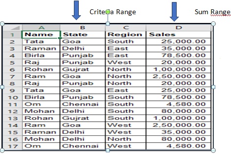
Now, in a particular cell where we need the sum total of sale for a particular state, say Goa, we will apply following formula in that cell

=+SUMIF(B:B,B2,D:D)

My range would be the whole column B, my criteria would be cell B2as it contains the state ‘Goa’ and my sum range would be whole column D.The resulting value would be 550000 and that is the total sale for Goa.

> SUMIFS Function

Similarly, the SUMIFS formula will return the sum value when there is more than one criteria. Taking the example of above table, if sales manager wants to know the total sale in the ‘North’ region of ‘Goa’. We can simply find out that by using filter, but again if we need the value in other worksheet for linking purpose and for further analysis, SUMIFS will work here. This function is used when there are large number of line items and the data is complex.

The Syntax is “=SUMIFS(sum_range, range1, criteria1, [range2], [criteria2], …)”

Now, in the cell where we require such value, we will apply below formula,

+SUMIFS(D:D,B:B,B2,C:C,C7)where the sum range is column D, my first criterion range would be column B as it consists the state, my first criteria would be cell B2 as it consists State ‘Goa’, my second criterion range would be column C as it consists the ‘Region’ and my second criteria would be cell C7 as it consists region ‘North’.

The result would be 250000 and that is the total sale in the north region of Goa.

> [INDEX + MATCH] Function

Index+Match function is very popular and quite common now in every type of industry. Basically, it is the substitute of the ‘vlook-up’ function. In ‘vlook-up’ function, there is a pre-condition that the unique value shall be at the left and this function will run from left to right in the worksheet. Whereas, in Index+Match function, no such condition is required.

In fact, this function is combination of two functions i.e. Index and Match. Sticking to the previous example, let’s insert one more column to the left of the first column and name it as ‘Category’ where we have put the category of each Salesman.

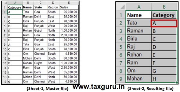
Sheet-1 is the master file and from this sheet, sales manager wants to know the categories of every salesman in Sheet-2.  Now, ‘vlook-up’ won’t work here as the ‘category’ column is on the left of the column ‘Name’. He can also do so by simply applying filter and Pivot as well for that matter. But if the manager wants it in another sheet i.e. in Sheet-2 and want to link it with the main sheet, the ‘filter’ function won’t work. And if he applies ‘Pivot’, then he has to refresh the Pivot data every time any update in the master file is done. Therefore, Index+Match is the best alternative.

First, we will use index function only. The Syntax is INDEX(array, row_num, [column_num]).

Index function will let us know the value which exist in a particular column and particular row. In Sheet 1, if we want to know the value in 5^th row and 1^st column, we will apply, =+INDEX(A1:E17,5,1) where A1:E17 is the selection of whole sheet, 5 is the row number and 1 is the column number. The resulting value will be ‘D’.

Now, we will use Match function. The Syntax is MATCH(lookup_value, lookup_array, [match_type]). Match function will let us know the position of a particular value in a row. For example, we want to know the position of value ‘D’ in first column of Sheet-1. We will apply the function, =MATCH(A5,A1:A17,0)where A5is the lookup value, A1:A17 is the lookup array and 0is the match type i.e. exact match. The resulting value is ‘5’. 

Now we can combine both the functionsand can get the desired result i.e. the category of each salesman. For Index function, we need the row number and column number which can be supplied by Match function, as we have seen above.

In sheet-2, we apply index+match function in cell B2 where we need to know the category of Mr. Tata. The formula is

“+INDEX(Sheet1!$A$1:$E$17,MATCH(Sheet2!A2,Sheet1!$B$1:$B$17,0),MATCH(Sheet2!$B$1,Sheet1!$A$1:$E$1,0))”

Where,

+INDEX(Sheet1!$A$1:$E$17	The selection of sheet where we need to find out the desired result
MATCH(Sheet2!A2,Sheet1!$B$1:$B$17,0)	We need to know the row number for Index function which we can get by applying Match function. We need to know the row number where ‘Tata’ Exist.
MATCH(Sheet2!$B$1,Sheet1!$A$1:$E$1,0)	We need to know the column number where ‘Category’ exist by applying Match function

The result will be ‘A’. We can now simply copy the function in other cells and get the desired result.

> Advance Filter

This function is advanced version of ‘Filter’ which we generally prefer to use. But in case of large data and if we want to use the filters simultaneously at some other place of the sheet, ‘Filter’ function will not be that useful. Although, advance filer has many feature, but here we will discuss only about filtering data and using it in some other place of sheet. The short-cut key of using the function is ‘Alt+A+Q’

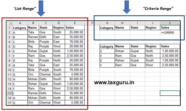
Sticking on the same example and table, suppose sales manager wants to know the salesman who made the sales Rs. 1 lakh or more. We can do the same by using traditional ‘Filter’ function and the result may be copied where we require such result. But ‘Advance Filter’ will solve our problem in much easier way.

Step-1: The first step is to specify the criteria. To do this, copy the headers and paste it somewhere else in the worksheet.

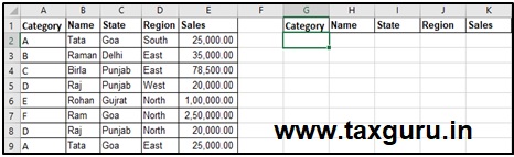
Step-2: Specify the criteria for which you want to filter the data. In this example, since we want to the sales more than or equal to 100000, enter >=100000 in the cell below Sales. This would now be used as an input in Advanced Filter to get the filtered data (as shown in the next steps).

Step-3: Press Alt, A, Q. and fill the following details in the Advance Filter dialogue box,

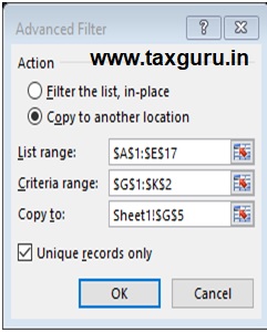
• Action:Select the ‘Copy to another location’ option. This will allow you to specify the location where you can get the list of unique records.
• List Range:Make sure it refers to the dataset from which you want to find unique records. Also, make sure headers in the data set are included.
• Criteria Range:Specify the criteria we constructed in the steps above. In this example, it would be G1:K2.
• Copy To:Specify the cell address where you want to get the list of unique records.
• Copy Unique Records Only:Check this option.
• Click OK.

We will get the desired result as below,

About the Author

Author is Amit Jindal, ACA working as Manager Taxation in Neeraj Bhagat & Co. Chartered Accountants, a Chartered Accountancy firm helping foreign companies in setting up business in India and complying with various tax laws applicable to foreign companies while establishing their business in India.