How to Use SUMIFS – Advance Excel

This article is inspired by my recent conversion with interviewer where he had asked after detailed technical round “Do you know Microsoft Excel and SUMIFS function”.

As usual I said yes I know.

And then I thought, is SUMIFS so important function in Microsoft Excel?? And if it is then I should write a detailed article on SUMIFS function.

In this article I will try to explain SUMIFS function in 5 different scenario from basic to advance.

For this Article you need to first download Microsoft Excel workbook of Sales Information of M/s XYZ Limited for the period of April-14 to March-16 attached herewith.  Download Excel Workbook

But before I proceed, I need to explain SUMIFS briefly how SUMIFS function works.

SUMIFS formula extends the abilities of a SUMIF function by giving us the facility to add only those items that meet a set of criteria.

SUMIF FUNCTION is work in this way

SUMIFS(Sum_Range, Criteria_Range1, Criteria1, [Criteria_Range2, Criteria2], …)

The SUMIFS function syntax has the following arguments

Sum_range:  Required, One or more cells to sum, including numbers or names, ranges, or cell references  that contain numbers. Blank and text values are ignored.

Criteria_range1:  Required, The first range in which to evaluate the associated criteria.

Criteria1: Required, The criteria in the form of a number, expression, cell reference, or text that define which cells in the Criteria_range1 argument will be added.

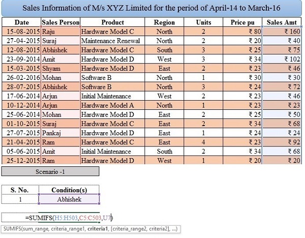
SCENARIO 1 – NEED TO GET SUM OF ALL SALES MADE BY ABHISHEK.

To get all sales made by Abhishek you need to just right simple SUMIFS Function

=SUMIFS(H5:H503,C5:C503,U7)

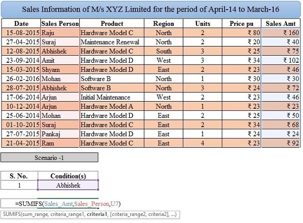
But wait we can write this formula in better way in understandable manner.

=SUMIFS(Sales_Amt,Sales_Person,U7)

You might ask how I did this, using name than ranges!!

Well, if you remember my article on Two Way Lookup I did the same thing. In my previous article where I created names for all numeric data values with their Top headings.

Same thing I also done here to create name of all data values with their respective headings.

If you are still confused let me repeat those three steps one again.

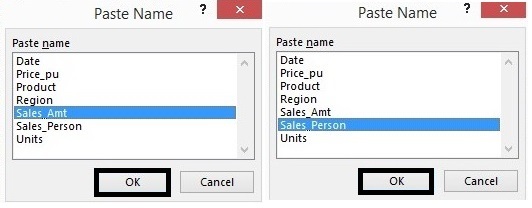
Steps 1 Select entire table (Short cut combination Ctrl + A)

Step 2 Go to the “Create from Selection” under “FORMALAS” tab (Short cut combination Ctrl +Shift + F3)

Step 3 Ensure that Top row is checked and click OK

Now while using SUMIFS write =SUMIFS(

Then press F3 (short cut key to display all names we created) and select Sales_Amt (Sum_Range) and press okay followed by, then again press F3 and select Sales_Person (Criteria_Range) followed by, and U7 (Criteria).

Instantly you will get same result with the use of name than range and, using meaningful range (Sales_Amt) is much more easier to remember than a range address (such as C5:C503) as well as make easier to use and understandable while using these name in formulas.

SCENARIO – 2 GET SUM OF ALL SALES MADE BY ABHISHEK FOR PRODUCT HARDWARE MODEL C.

For this scenario we just need to expand our formula by adding one more criteria range (Product) and criteria (Hardware Model C)

=SUMIFS(Sales_Amt,Sales_Person,U7,Product,U8)

 SCENARIO – 3 GET SUM OF ALL SALES MADE BY ABHISHEK FOR PRODUCT HARDWARE MODEL C IN SOUTH REGION.

Again we just need to expand our formula by adding one more criteria range (Region) and criteria (South)

=SUMIFS(Sales_Amt,Sales_Person,U7,Product,U8,Region,U9)

 

 SCENARIO – 4 GET SUM OF ALL SALES MADE BY ABHISHEK FOR THE PERIOD APRIL 15 TO MARCH 16.

This is tricky, in all other previous scenarios we have to get calculate sum based on single criteria but in this case we need to compute sum on the basis of range.

And for these types of problems we need to understand comparatives operators of Microsoft Excel.

Description	Symbol	Description	Symbol
Greater than	>	Greater than or equal to	>=
Less than	<	Less than or equal to	<=
Equal to	=	Doesn’t equal to	<>

Now come back to our Scenario 4, where we have to need a sum of all sales made by Abhishek during the period of April15 to March16.

In this case we need to use comparative operator “>=” greater or equal before 01-04-2015, since we need information of all sales made on or after 01-04-2015. And “<=” less than or equal to before 31-03-2016, since we don’t want to have any information of sales made on after 31-03-2016.

And or formula will be

 =SUMIFS(Sales_Amt,Sales_Person,U7,Date,U8,Date,U9)

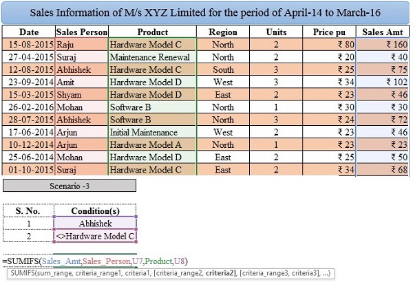
SCENARIO – 6 GET SUM OF ALL SALES MADE BY ABHISHEK OTHER THAN PRODUCT HARDWARE MODEL C.

This again requires comparative operator “<>” does not equal to product Hardware Model C, since we don’t want sales information of “Hardware Model C”. Therefore we need to use “<>” to validate our conditions.

And our formula will be

=SUMIFS(Sales_Amt,Sales_Person,U7,Product,U8)

There are N number of situation we can create, which we generally have to face in our daily routine office work. And you might have your own short cuts and tricks to deal with these situations, but when you are aware and regularly using these comparative operators in between normal Microsoft Excel formulae, you will start playing with Microsoft Excel or sometime you will able to write your own Complex Excel Formulae.  And important thing is theses comparative operations not only in SUMIFS Function, you may use in SUMIF, COUNTIF, COUNTIFS AND EVEN IN VLOOKUP too. You need to just try.

Anyway, now I can assume you all are aware about how to use these comparative operations, so that I could avoid to explain these in my future articles.

Hope you all are gain something from this article and if we have any query regarding this article or anything regarding Microsoft Excel feel free to comment or get in touch.

(Author can be reached at camukeshkumar@outlook.com)